
Double-Clip MGDA: Clipping Away Double Sampling
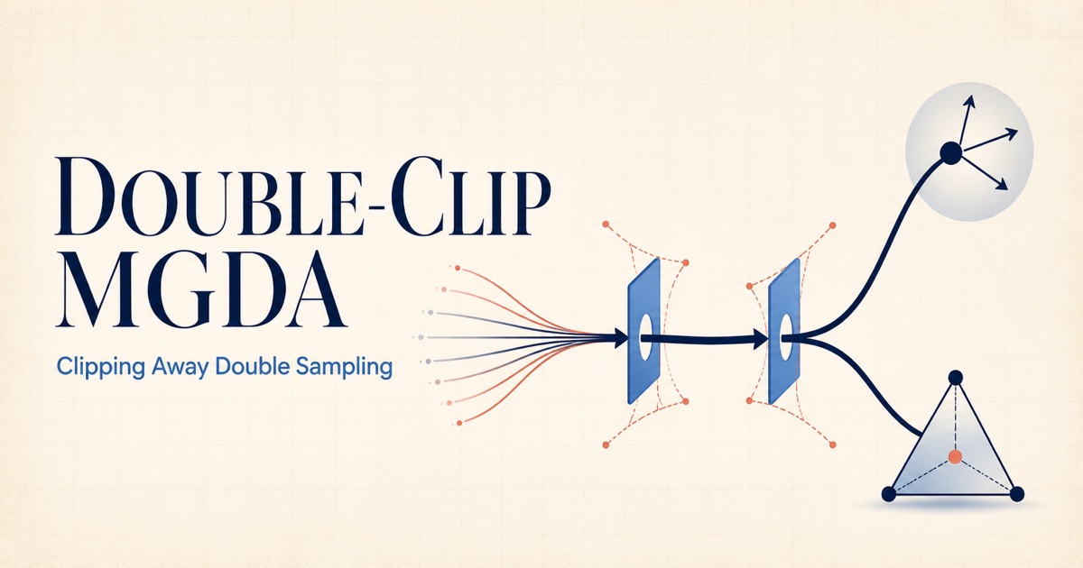
The main idea is unexpectedly simple: clip the balanced gradients, then reuse the same clipping factors in the model, dual, and preference updates. That coupling removes the need for double sampling, a bias-control strategy used to obtain convergence guarantees for stochastic MGDA-type methods with static batch sizes (Chen et al., 2024; Xiao et al., 2023).
Algorithm 2, first
Consider $m$ robust objectives. The algorithm maintains three objects:
- $\theta_t$: the shared model parameters;
- $\eta_t$: one dual variable per objective, introduced by the distributionally robust reformulation;
- $w_t \in \mathcal W$: a preference vector on the probability simplex, so $w_t \ge 0$ and $\mathbf 1^\top w_t=1$.
Let $\widehat{\mathcal L}(\theta,\eta)$ denote the paper’s rescaled vector of dual objectives. At iteration $t$, $Z_t$ collects its stochastic gradients with respect to the dual variables and $X_t$ collects its stochastic gradients with respect to the model. Algorithm 2 is:
The order is deliberate. Here is what each block does.
Lines 4–5: update the dual variable first
The dual variable $\eta_i$ is the finite-dimensional stand-in for the worst-case distribution of objective $i$. Line 4 estimates all dual gradients at the current pair $(\theta_t,\eta_t)$. Multiplying by $w_t$ forms the balanced dual direction $Z_tw_t$, and $\mu_t$ clips that direction before the step:
\[\lVert \gamma \mu_t Z_tw_t\rVert \le \gamma f_2.\]This is not an inner optimization loop. It is one dual step per outer iteration. Objectives with larger current preference receive proportionally more influence through $w_t$, while clipping prevents an unstable dual direction from dominating the dynamics.
This dual-first clipped update is a direct generalization of the single-objective D-SGD-C design of Zhang et al. (2025) to preference-weighted multi-objective dynamics. We refer interested readers to that paper for the single-objective proof intuition and to Corollaries K.6–K.8 of our paper for the corresponding multi-objective generalization along the sequential trajectory.
Lines 6–7: use the new dual state to update the model
Only after computing $\eta_{t+1}$ do we evaluate $X_t$. In other words, the model gradient is measured at $(\theta_t,\eta_{t+1})$, not at the stale dual state. This sequential, Gauss-Seidel-like order is important: the model immediately responds to the latest approximation of each objective’s adverse distribution.
The balanced model direction is $X_tw_t$. Its clipping factor $\alpha_t$ gives the analogous bound
\[\lVert \gamma \alpha_t X_tw_t\rVert \le \gamma c_2.\]Thus both sides of the ill-conditioned geometry—the dual variables and the model parameters—move on controlled scales.
Line 8: make the preference update obey the same geometry
Ordinary MGDA chooses $w$ to make the balanced gradient small. A projected gradient step for the model-gradient term naturally contains $X_t^\top X_tw_t$. In DR-MOO, stationarity also needs the dual component, which contributes $Z_t^\top Z_tw_t$.
The crucial detail is that line 8 does not use the raw Gram terms. It uses the same $\alpha_t$ and $\mu_t$ that controlled the parameter steps:
\[\underbrace{\alpha_tX_t^\top X_tw_t}_{\text{model balance}} \;+ \underbrace{\mu_tZ_t^\top Z_tw_t}_{\text{dual balance}} \;+ \underbrace{\rho w_t}_{\text{regularization}}.\]Finally, $\Pi_{\mathcal W}$ projects the result back to the simplex, keeping the preferences nonnegative and summing to one. This shared scaling is the heart of Double-Clip MGDA: the preference vector is trained using the same bounded geometry that actually moves $\theta$ and $\eta$.
The generic form: no dual variable required
The mechanism is not restricted to DRO. For ordinary stochastic objectives collected in the vector $\mathbf F(\theta)$, start from Algorithm 2 and delete the dual variable $\eta_t$, the dual-gradient matrix $Z_t$, the clipping factor $\mu_t$, and every update involving them. The entire generic method can then be written as one algorithm:
When $X_tw_t=0$, take $\alpha_t=c_1$. The same balanced-gradient clip is used twice: once in the model update and once in the preference-vector update. This primal-only framework is therefore Algorithm 2 with all dual-variable components removed.
Proof intuition: why coupled clipping works
The usual stochastic MGDA preference step contains a one-batch Gram term such as $X_t^\top X_tw_t$. Because $\mathbb E[X_t^\top X_t]\ne(\mathbb E X_t)^\top(\mathbb E X_t)$, a standard bias-control device forms the product from two independent gradient batches. Double-Clip MGDA keeps one Gram estimate and controls its contribution instead. The proof is easiest to understand through two ideas.
1. Decouple problem constants from the clipping radius
The caps $c_1,f_1$ and radii $c_2,f_2$ are explicit algorithmic controls; they are not hidden inside smoothness, variance, or gradient-bound constants. Because
\[\alpha_t\lVert X_tw_t\rVert\le c_2, \qquad \mu_t\lVert Z_tw_t\rVert\le f_2,\]the model and dual steps are bounded by $\gamma c_2$ and $\gamma f_2$. Reusing those same factors in the $w_t$ update also keeps the parameter dynamics and preference-vector dynamics on comparable scales. In Theorem 5.2, the choice $c_1=f_1=1/2$ and $c_2=f_2=\delta\epsilon$ makes the target accuracy enter through the clipping radii while allowing $\beta$ and $\gamma$ to remain order-one. This separation is what makes the magnitude controllable across $\theta_t$, $\eta_t$, and $w_t$.
2. Prove descent in the metric created by clipping
Expanding the projected preference update, as in Eq. (85) of Lemma L.2, produces the useful inner products
\[-2\beta\alpha_t\langle w_t-w,X_t^\top X_tw_t\rangle -2\beta\mu_t\langle w_t-w,Z_t^\top Z_tw_t\rangle,\]along with quadratic remainder terms such as
\[\beta^2\alpha_t^2\lVert X_t^\top X_tw_t\rVert^2, \qquad \beta^2\mu_t^2\lVert Z_t^\top Z_tw_t\rVert^2.\]The normalization in $\alpha_t$ and $\mu_t$ is exactly what controls these remainders. Schematically,
\[\alpha_t^2\lVert X_t^\top X_tw_t\rVert^2 \le c_2^2\lVert X_t\rVert_F^2, \qquad \mu_t^2\lVert Z_t^\top Z_tw_t\rVert^2 \le f_2^2\lVert Z_t\rVert_F^2.\]After scaling Eq. (85) and combining it with the sequential trajectory
\[(\theta_t,\eta_t)\longrightarrow(\theta_t,\eta_{t+1}) \longrightarrow(\theta_{t+1},\eta_{t+1}),\]the analysis does not try to isolate a raw population quantity like $\lVert\nabla\widehat{\mathcal L}\,w_t\rVert^2$. Instead, it obtains descent directly in the clipped metric
\[\gamma\alpha_t\lVert X_tw_t\rVert^2 +\gamma\mu_t\lVert Z_tw_t\rVert^2.\]This is the key match: the proof measures progress in the same geometry that the algorithm actually uses.
For the stochastic cross terms, write
\[\widehat\Gamma_t=X_t-\nabla_\theta\widehat{\mathcal L}(\theta_t,\eta_{t+1}), \qquad \widehat\Upsilon_t=Z_t-\nabla_\eta\widehat{\mathcal L}(\theta_t,\eta_t).\]Adding and subtracting these population gradients decomposes the mixed terms in Eqs. (89)–(90). Cauchy–Schwarz then leaves expressions controlled directly by $\alpha_t\lVert X_tw_t\rVert$ or $\mu_t\lVert Z_tw_t\rVert$. Since $c_2=f_2=\delta\epsilon$, the preference-update remainders acquire an explicit $\delta^2\epsilon^2$ factor. They can be absorbed into the clipped descent bound without an independent Gram estimator and without forcing $\beta=O(\epsilon^2)$.
That is why this is a genuinely multi-objective argument. In a single-objective method there is no preference-vector trajectory, so neither the $w_t$ coupling terms nor this clipped preference descent exists. The result depends on clipping all three coupled dynamics—model, dual, and preference—not on importing a single-objective clipping proof.
Under the paper’s assumptions, this produces a single-loop method with $O(\epsilon^{-4})$ sample complexity, matching the sample complexity that a stochastic first-order algorithm without variance reduction can achieve Arjevani et al. (2023). The theory requires batch size of order $O(\epsilon^{-2})$; in the reported ablation, a batch size of 256 was already sufficient for stable behavior.
Experimental results
We used a pretrained ResNet-18 encoder with task-specific MLP heads, cross-entropy loss, and the dual of a $\chi^2$-divergence robust objective. Every baseline optimized the same dual DR-MOO formulation, with its hyperparameters tuned.
Multi-MNIST: test accuracy under FGSM attack
The table below reports the accuracy values from Table 1 of the paper without additional aggregation or interpretation.
| Method / Attack Level | Multi-MNIST 2-digits (70-epochs training) | Multi-MNIST 3-digits (100-epochs training) | ||||||||
|---|---|---|---|---|---|---|---|---|---|---|
| 0.00 | 0.01 | 0.03 | 0.05 | 0.08 | 0.00 | 0.01 | 0.03 | 0.05 | 0.08 | |
| Double-Clip MGDA | 95.66% | 83.48% | 65.95% | 60.40% | 57.13% | 98.76% | 97.59% | 94.40% | 91.05% | 86.65% |
| Double-loop MGDA | 92.80% | 72.81% | 57.71% | 54.49% | 51.63% | 97.49% | 95.38% | 89.99% | 85.25% | 79.88% |
| MoCo | 94.49% | 77.69% | 61.74% | 58.63% | 56.43% | 98.27% | 96.62% | 92.75% | 88.75% | 83.43% |
| NashMTL | 91.21% | 62.58% | 51.67% | 49.54% | 47.09% | 96.17% | 92.31% | 84.53% | 78.91% | 73.48% |
| FAMO | 89.05% | 61.04% | 50.82% | 48.66% | 46.48% | 95.90% | 91.86% | 84.29% | 78.94% | 73.52% |
| SDMGrad | 89.59% | 64.02% | 52.00% | 49.91% | 47.31% | 96.46% | 92.89% | 85.06% | 79.37% | 73.50% |
| MoDo | 91.10% | 64.08% | 51.95% | 49.73% | 47.49% | 96.50% | 93.15% | 86.03% | 80.56% | 74.81% |
| MGDA | 89.44% | 62.61% | 52.19% | 50.81% | 48.30% | 96.34% | 92.85% | 85.42% | 80.26% | 75.18% |
CelebA: robustness to task-wise label imbalance
Double-Clip MGDA also led every aggregate metric on CelebA. All entries are percentages averaged across tasks.
| Method | Average accuracy | Balanced accuracy | AUC |
|---|---|---|---|
| Double-Clip MGDA | 88.41 | 89.55 | 94.63 |
| Double-Loop MGDA | 86.61 | 87.97 | 93.28 |
| MoCo | 87.27 | 88.50 | 93.31 |
| NashMTL | 85.58 | 87.00 | 92.41 |
| FAMO | 85.32 | 86.03 | 91.41 |
| SDMGrad | 85.89 | 87.06 | 92.45 |
| MoDo | 85.66 | 87.08 | 92.42 |
| MGDA | 85.53 | 86.87 | 92.58 |
Optimization and ablation evidence
The synthetic linear-regression and white-wine logistic-regression studies tell a complementary story: both proposed methods were competitive in balanced-gradient convergence, while Double-Clip avoided the expensive inner loop. The batch-size ablation also showed the practical trade-off predicted by the theory—small batches fluctuated, and the instability became negligible around batch size 256.
References
-
Lisha Chen, Heshan Fernando, Yiming Ying, and Tianyi Chen. “Three-Way Trade-Off in Multi-Objective Learning: Optimization, Generalization and Conflict-Avoidance.” Journal of Machine Learning Research 25(193), 1–53, 2024.
-
Peiyao Xiao, Hao Ban, and Kaiyi Ji. “Direction-Oriented Multi-Objective Learning: Simple and Provable Stochastic Algorithms.” Advances in Neural Information Processing Systems 36, 4509–4533, 2023.
-
Qi Zhang, Yi Zhou, Simon Khan, Ashley Prater-Bennette, Lixin Shen, and Shaofeng Zou. “Revisiting Large-Scale Non-Convex Distributionally Robust Optimization.” International Conference on Learning Representations, 2025.
-
Yossi Arjevani, Yair Carmon, John C. Duchi, Dylan J. Foster, Nathan Srebro, and Blake Woodworth. “Lower Bounds for Non-Convex Stochastic Optimization.” Mathematical Programming 199, 165–214, 2023.
More benchmarks are coming
These results are the first benchmark suite, not the last. We plan to add broader datasets, architectures, objectives, and stronger MOO baselines as we continue studying the algorithm. The especially interesting question is whether the primal-only form above can provide the same stability benefits outside distributionally robust objectives.
If you use Double-Clip MGDA, or build a new MOO method from its balanced-gradient clipping idea, please cite our paper:
Yufeng Yang, Fangning Zhuo, Ziyi Chen, Heng Huang, and Yi Zhou.
“Distributionally Robust Multi-Objective Optimization.” arXiv:2605.05660, 2026.
Paper · DOI
@misc{yang2026distributionallyrobustmoo,
  title         = {Distributionally Robust Multi-Objective Optimization},
  author        = {Yang, Yufeng and Zhuo, Fangning and Chen, Ziyi and
                   Huang, Heng and Zhou, Yi},
  year          = {2026},
  eprint        = {2605.05660},
  archivePrefix = {arXiv},
  primaryClass  = {cs.LG},
  doi           = {10.48550/arXiv.2605.05660}
}